TableSkim draws charts of the rows you are looking at and summarizes them in tables, without a spreadsheet or a script. This page shows, with examples, which tool answers which question, how to read the result, and how to go from a chart to the rows behind it. The examples use the demo files in demo/examples/: iris.csv (150 flowers), penguins.csv (344 penguins), and hour.csv.xz (17,379 hourly bike rental records). See Example datasets for sources, units and how to open them.
| Question | Tool | GUI | TUI |
|---|---|---|---|
| What values does a column hold, and how many of each? | Histogram | Edit → Histogram... | B |
| Are two number (or date) columns related? | Scatter plot, density | Edit → Scatter Plot... | M |
| How does a number differ between groups? | Box plot | Scatter Plot, text on X | M |
| How many rows, and what totals or averages, per group? | Group By | Edit → Group By... | A |
| Minimum, maximum, mean of one column? | Column statistics | Edit → Column Statistics | S |
Every tool works on the current view: the rows left by the filter. So you can filter first (for example to one year) and then chart or group just those rows; the charts follow when the filter changes.
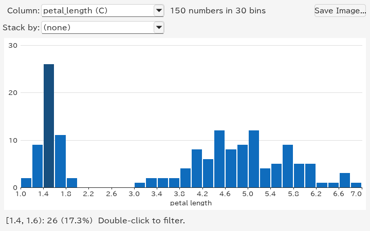
A histogram counts how many values fall into each range ("bin") of a column. Put the current cell in the column and choose Edit → Histogram... (Ctrl+Shift+H).
How to read it:
[1.4, 1.6): 26 (17.3%): 26 flowers have petals at least 1.4 cm and less than 1.6 cm long.
Dates are counted into whole days, months or years; a column of text shows its most frequent values instead, longest bar first. Stack by another column (species, say) splits each bar by that column's values, in a colour for each, so that you can see what each range is made of. See Histograms for every option and How bins are chosen for the details.
A scatter plot draws one point per row, with one column across (X) and another up (Y). Choose Edit → Scatter Plot... (Ctrl+Shift+P). Select two columns first to plot exactly those (the first one is X); otherwise TableSkim picks number or date columns near the current cell, and you can change them in the X and Y lists.
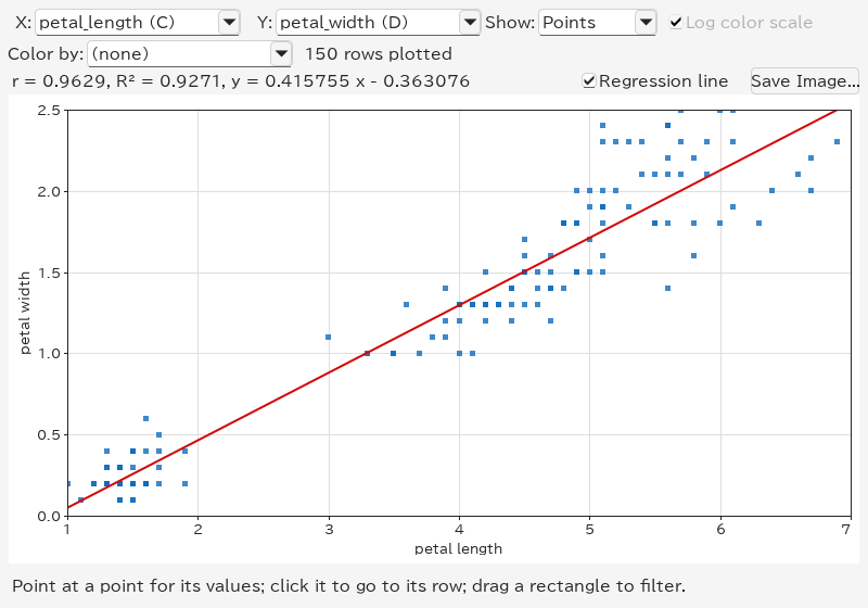
How to read it:
r ≈ 0.9629: longer petals tend to be wider.
y = 0.4158 x − 0.3631, with both lengths in cm. This describes an association, not causation.
species, say) gives each of its values a colour, with a legend above the plot, so that you can see whether the groups lie apart. Click an entry of the legend to filter to its rows.
The overall Iris correlation also reflects differences between species; filter to one species to study the relationship within it.
With many rows, points pile up on each other. Show → Density counts the rows in a grid instead, and colours each cell from dark (few rows) to yellow (many):
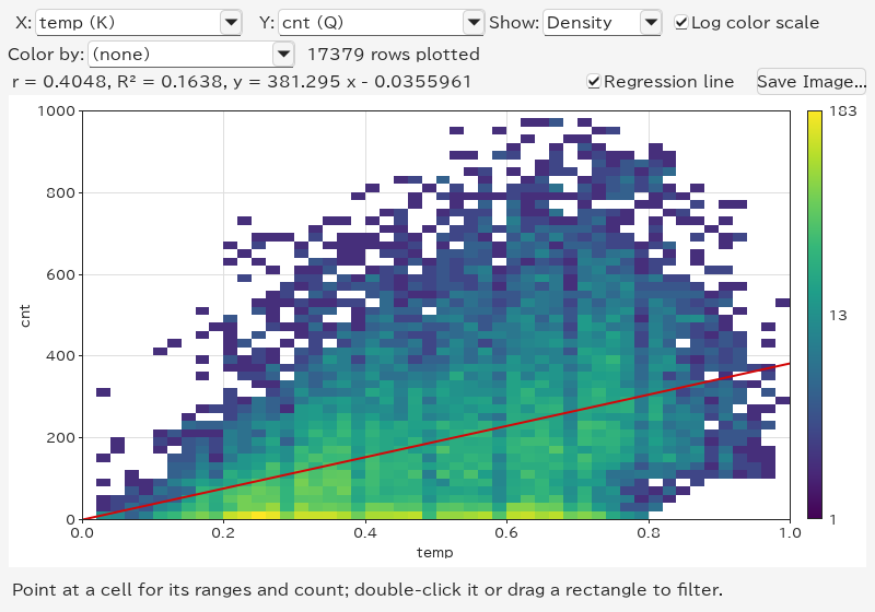
This example uses Bike Sharing: X → temp, Y → cnt. Temperature is normalized, not in degrees Celsius; cnt counts rentals in an hour. Demand also changes with hour, season and working day, so temperature alone does not explain it. Log color scale keeps cells with a handful of rows visible next to the busiest ones; turn it off to compare counts linearly.
When X is a column of text, such as species, each of its values becomes a group with a column of its own, and the plot shows a box plot per group. Here: X → species, Y → petal_length in Iris.
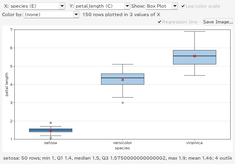
How to read a box:
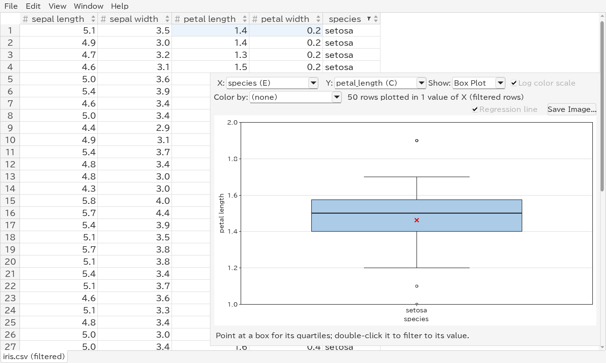
Setosa has the shortest petals (median 1.5 cm), versicolor lies between (median 4.35 cm), and virginica has the longest (median 5.55 cm). Each species has 50 flowers. Up to 30 groups are shown, the largest first; the rest are drawn together as (other).
For a group with more than 1,048,576 values, the box statistics are estimated from a uniform sample of that many values. The displayed row count still includes the whole group; the sample size and an estimate label appear with the box's numbers. Minimum, maximum and outlier counts also describe the sample. Density counts use all rows. The sample is the same whether points are retained or only the density is calculated.
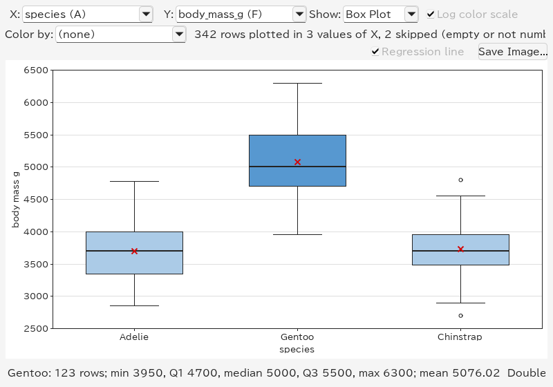
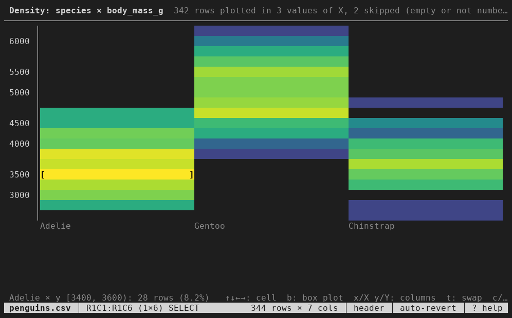
For another example, open penguins.csv, with X → species, Y → body_mass_g. Gentoo penguins are generally heavier than Adelie and Chinstrap. Two rows have no body mass and are skipped; 342 are plotted.
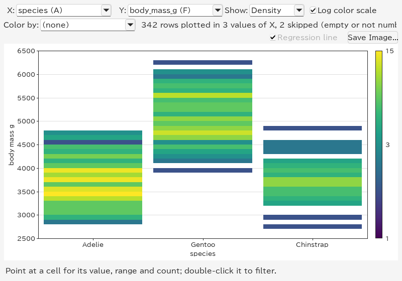
Show → Density shows each group's histogram as a column of coloured cells, which tells more about the shape than a box (two peaks, say):
Charts show patterns; Group By gives the numbers. Edit → Group By... (Ctrl+Shift+G) asks which columns to group by and which to summarize, and puts the result in a new sheet named Group By.
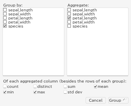
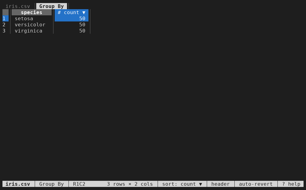
Check only a column to group by and press Group: the result has one row per value with its count. Sort the count column (click its sort button twice) to see the largest groups first:
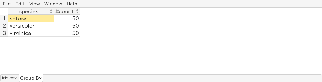
The result has three rows: setosa, versicolor and virginica, each with count = 50. There is no empty species in Iris.
Check columns under Aggregate and the functions below: count (values that are not empty), distinct (different values), sum, mean, min, max and std dev (standard deviation). Each aggregated column and function gives a column such as petal_length mean. Means often have many decimals; Format in the column header menu shows them rounded, for example to three decimal places:
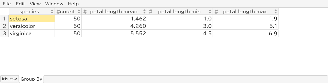
The means are 1.462 cm (setosa), 4.260 cm (versicolor) and 5.552 cm (virginica). These numbers summarize the differences shown in the boxes.
Leave every Group by column unchecked: all rows form one group, and the result is one row of totals:

Check two or more Group by columns to count each combination, for example species and island in penguins.csv: a row for each species–island combination.
The Group By sheet is an ordinary sheet: sort it, filter it, chart it (a histogram of count, say), copy it, or save it with File → Export View.... Grouping again replaces it. It stays when the file is reloaded, but it does not change when the original sheet does; group again after changing the filter. See Group By for how values are compared.
Charts and filters work together, so you can drill down step by step:
Double-clicking the setosa box above leaves its 50 flowers:
Save Image... in the histogram and scatter plot windows writes the chart as shown, with its axis titles, to a file:
.png): a picture at the size of the window, for slides, documents and chat.
.svg): lines and text stay sharp at any size, and the file can be edited in a vector drawing program. The points of a scatter plot are a picture inside it.
The type follows the extension you type, or the type chosen in the file dialog. Resize the window first to change the size of the image.
In the web app, Save PNG and Save SVG in the chart dialogs do the same; the browser saves the file into its downloads. The points of a scatter plot are separate shapes in its SVG.
The terminal UI has the same tools, drawn with characters:
B shows a histogram of the cursor's column; Enter filters to a bar, and g / G stack its bars by another column.
M shows the density of two columns (select them first), or box plots when X holds text; b switches between the box plots and the density, Enter filters to a box or cell.
A opens the Group By dialog; the result is a sheet, which o sorts.
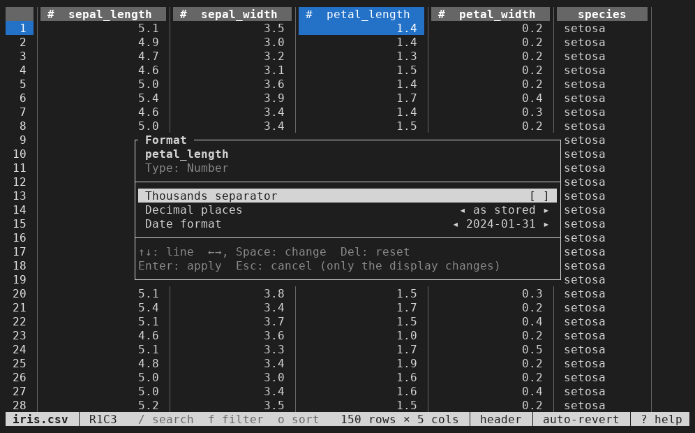
% formats the current column, as Format does in the GUI.
See Using the Terminal UI for all keys. Saving charts as images is available in the GUI only.